FT-ICR.
Like so many scientific acronyms, this one is gibberish to most lay people. The translation – Fourier Transform Ion Cyclotron Resonance – probably wouldn’t help them much either. But there’s a lot going on in those five little letters, particularly at the MagLab, a world leader in the field and home to the man who co-invented the technique and, more than anybody else in the past three-plus decades, is responsible for the great advances in chemistry that have been made through its use.
Chief Scientist for Ion Cyclotron Resonance Alan Marshall
FT-ICR is a very special type of mass spectrometer (a machine that measures the mass of atoms and molecules). In fact, this extremely powerful tool offers much more accurate and precise measuring than any other type of mass spectrometer (MS for short).
Why measure the mass of atoms and molecules in a substance? To find out what it’s made of – which atoms, which molecules and how much of each. This information can speak volumes about the origin and properties of a substance.
The field of FT-ICR is one of the greatest strengths of the National High Magnetic Field Laboratory. For one, our facilities are unrivaled. Our ICR Facility includes several FT-ICR mass spectrometers, including the most powerful one in the world, which uses a superconducting magnet with a field of 21 tesla. Tesla is a measurement of the strength of a magnetic field: To put that in perspective, 1 tesla is equal to 20,000 times the Earth's magnetic field.
Before amassing the hardware, though, FSU started with superb talent. The ICR Facility was founded by Chief Scientist for Ion Cyclotron Resonance Alan Marshall, a legend in the field. Along with Melvin Comisarow of the University of British Columbia in Canada, Marshall invented the FT-ICR back in 1973. The feat dates back to 1931, when the ion cyclotron, a device that accelerates negatively or positively charged particles (ions) in a magnetic field, was invented. The tool was adapted to create the ion cyclotron resonance mass spectrometer a few decades later. Fourier transform (a mathematical algorithm that converts signals detected over time into a spectrum of usable data about, say, particle mass) has been around for centuries. But Marshall and Comisarow were the first to put two and two together (or rather, FT and ICR together) and create an amazingly powerful device. These machines are used for all types of research, from studying how drugs and cells interact to analyzing the more than 30,000 chemical substances in a single heavy petroleum sample. No wonder that more than 650 mass-spectrometry instruments based on Marshall’s three patents have been installed worldwide, with about 50 new ones going online every year.
FT-ICR is the best technique by far for analyzing complex molecules mixed together in a fluid – which is how molecules are often found. But before we launch into a blow-by-blow of how this works, let’s first address how it matters.
Cracking the Code
Let’s say you’re contemplating drilling for oil far out at sea – an increasingly familiar scenario to oil companies that have exploited all the easily accessible reserves. This undersea stash will be awfully difficult – and expensive – to get to. Is it worth it?
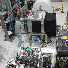
A group member working in the ICR facilities.
To find out, you extract a drop of it and send it to the MagLab. After all, it was here that the micro-analytical study of these substances – petroleomics – was born.
To you, all crude oil might look, smell and feel the same. And in fact, all crude oil is made up mostly of hydrocarbons, molecules of carbon and hydrogen. But on a molecular level, there can be tremendous differences. There are many types of hydrocarbons, for example. Crude oil contains varying amounts of nitrogen, sulfur, nickel and other elements, as well. The makeup depends on where, and under what pressures and temperature, it was formed, as well as the types of plants that decomposed to make it.
In fact, crude oil is supremely complex – one sample might contain more than 30,000 different chemical substances. Those molecules harbor important information – about the sample’s tendency to rust steel pipes or to clog them (corrosivity), for example, or what makes it form an emulsion with water. A close look at the content of sulfur, a pollutant, in the oil would indicate how difficult it would be to get rid of. Having such detailed chemical profiles of crude oil could also help pinpoint the origin of a spill.
Weighing In
When scientists want to figure out what something is made of, on the molecular level, they weigh it. Your bathroom scale won’t do: molecules just don’t seem to register on them. So they use mass spectrometers instead. There are lots of different types, each offering its own advantages (for a discussion on MS basics and details on a type of MS designed at the lab to weigh comet dust, please see our Magnet Academy article Mass Spectrometry 101). But when it comes to sorting out substances that are exceptionally complex, scientists usually opt for FT-ICR.
Each atom has a distinct atomic mass (also called atomic weight), which is a function of the number of its protons and neutrons. A carbon atom, for example, weighs 12.011 Daltons (the unit of mass for atoms). A tin atom weighs 118.69.

Actually, that’s a lie. There’s not a single tin atom in the universe that weighs 118.69. Some weigh 116, some 118, some 120, to name a few. These are all different isotopes – atoms of the same element that vary in the number of neutrons in their nuclei, and hence in their mass (most elements don’t have as many isotopes as tin does). The atomic mass listed on the periodic table is a weighted average of the masses of all the naturally occurring isotopes of a chemical element.
One challenge of MS is to tell such isotopes apart, starting with the lightest – hydrogen isotopes weighing in the neighborhood of 1 Dalton. But big, cumbersome molecules also pose a substantial challenge. They may contain upwards of 1,000 atoms, which translates into atomic masses that exceed 100,000 Dalton! That’s a phenomenal range, and measuring accurately from one extreme to the other is a very tall order.
FT-ICR is up to the task.
Ready for our Close-Up
Sometimes the difference between the masses of two isotopes, or two molecules, is quite tiny. This is where resolution power makes all the difference in mass spectrometry. It’s like having a camera with a series of super duper zoom lenses. The more you zoom, the more you see. If all you’ve got to work with, though, is a cheap disposable, you’re not going to capture much detail.
Take the series of images below, for instance. The first is an oak leaf. Examine it more closely, though, and you'll see it's made up of cells. Look even closer, and you'll see inside each cell a nucleus. (These images, by the way, come from an outstanding tutorial well worth checking out called Secret Worlds: The Universe Within, which explains the powers of 10. It's found on the excellent microscopy Web site, Molecular Expressions).

The closer you look, the more you see.
Get the picture? Now, let's transfer this concept to mass spectrometry, viewing the next three images in the same way as you've just examined the above three images.
Take a look at the graph below, which depicts the MS results of a sample of South American crude oil.
Broadband mass spectrum of a crude oil sample.
This is a mass spectrum, the type of reading you’ll get from any mass spectrometer. Each peak represents a type of atom or, in this case, molecule. The numbers running across the bottom of the graph – what’s called the mass to charge ratio, or m/z – refer to the molecule’s atomic mass. The height of the peaks tells us how many there are.
As you can see, these peaks are packed in pretty densely. In the example, the range of molecular masses covered starts at about 225 Dalton and goes up to 1,000 Dalton – and there’s an awful lot happening in between. The crude oil is complex; it’s hard to differentiate the molecules.
Zoom in a bit closer, though, and you can see a lot more.

Enlarged region of the mass spectrum of a crude oil sample.
We’ve honed in significantly on our sample here, covering not a range of 775 Dalton but of 50. It becomes clear that the blur we saw in the broadband spectrum actually can be broken down into individual, discernible peaks – just as the leaf is broken down into discrete cells.
However, the lines are still pretty fuzzy. To be able to tell those peaks apart – or even to know that there is more than one peak there – we need to zoom in even closer. Let's pull out a magnifying glass and examine the area around the 426 Dalton mark.
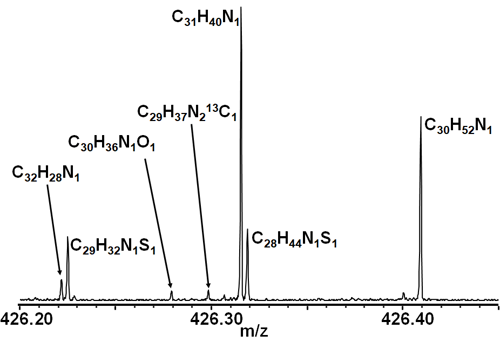
Enlarged region of the mass spectrum of a crude oil sample, identifying individual hydrocarbons.
Aha! What before looked to be a single line is actually several, depicting several separate hydrocarbons. C31N40N1 is the most numerous of the bunch, but the sample also contains (in order of abundance), C30H52N1, C28H44N1S1 and C29H32N1S1, among others. Like the leaf cell nuclei in the example above, these peaks emerge under the FT-ICR microscope to reveal what's really going on.
In fact, when you look at this crude oil sample with the help of FT-ICR, you will find upwards of 11,000 different hydrocarbons.
Other machines cannot produce this level of detail. Instead, they essentially lump together several different molecules in a single peak, which represents their weighted average – something quite different than what is truly there. This capacity is of extreme interest to scientists, and something the MagLab does exceptionally well. In fact, the instruments here hold the world record in mass resolution! You may be surprised to hear that such a thing exists, but MagLab scientists were able to differentiate between two distinct molecules that were only about 0.000452 Dalton apart in atomic mass. That’s about as much as an electron weighs, which is so close to nothing as to boggle the mind.
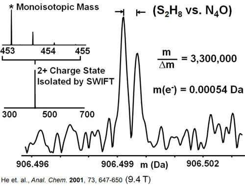
World record for mass resolution.
Horseshoes and Hand Grenades
We’ve talked about the high resolution powers of FT-ICR. Let’s take a minute to admire its high mass accuracy.
Mass spectrometers, including FT-ICR, often don’t hit a bull’s eye when they’re measuring mass. Sometimes, pretty close is close enough: given the sample, you can be reasonably sure what the substance is. Sometimes, pretty close doesn’t cut it.
Let’s take another look at the crude oil sample from the previous section.
Enlarged region of the mass spectrum of a crude oil sample, identifying individual hydrocarbons.
Now let's look at the weights of the hydrocarbons identified above, as determined by FT-ICR.
| Chemical Formula |
Measured Mass |
Calculated Mass |
| C32H28N1 |
426.22177 |
426.22163 |
| C29H32N1S1 |
426.22511
|
426.22500
|
| C30H36N1O1 |
426.27925
|
426.27914
|
| C29H37N213C1 |
426.29854
|
426.29848
|
| C31H40N1 |
426.31562
|
426.31553
|
| C28H44N1S1 |
426.31895
|
426.31890
|
| C30H52N1 |
426.40949
|
426.40943
|
Look at C31H40N1 (fifth from the top). The actual mass of this hydrocarbon (at least as best as scientists can determine) is 426.31562 Dalton. A less accurate type of MS would give you a reading of 426, or maybe 426.3. Clearly, that’s not accurate enough to distinguish this molecule from others in the sample, such as nearby C28H44N1S1, with a mass of 426.31895 Dalton. A reading to the next decimal spot would also be iffy in some instances.
FT-ICR can determine masses five figures past the decimal point. With this kind of accuracy, it is possible to determine beyond the shadow of a doubt the identity of unknowns, based simply on mass. This accuracy is all the more impressive when you consider that the machine is not just weighing one element at a time, but may well be measuring upwards of 10,000 elements at once (as in this example), and can determine the composition of each of them with extremely high confidence.
Also of great importance is that FT-ICR MS can simultaneously separate and identify great numbers of substances – more than 10,000 separate chemical constituents within a single sample. Other mass analyzers are unable to cover such a vast spectrum.
Finally, unlike other MS methods, FT-ICR doesn’t destroy molecules in the measuring process (we’ll see this shortly, when we discuss how the machine works). That means you can use them again. For example, after measuring the molecules once, you can break them down into smaller pieces, and remeasure those pieces for a new level of information on the sample.
Charge It!
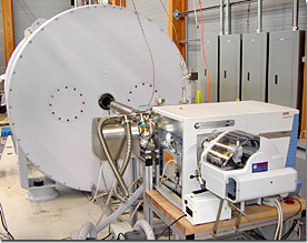
The Magnet Lab's 14.5 tesla, 104 mm bore FT-ICR system.
Now for a look at one of these mass measurement marvels.
Pictured on this page is the MagLab's 14.5 tesla, 104 mm bore FT-ICR system. Though you can't tell much by looking at it from the outside, wonderful things happen on the inside that reveal amazing details about the sample being studied.
First off, though, the sample molecules need to be ionized – that is, turned into a charged particle. That charge – positive or negative – makes the molecule react to the magnetic field of the device. This is the core principle behind any mass spectrometer: Each type of ion will respond differently to that magnetic field, depending on its mass. There are various methods of ionization, each offering its own advantages.
After the molecules are ionized, they are funneled by an ion guide into the analyzer cell (also called a Penning trap), which is located in the center, or bore, of a superconducting magnet. This whole set-up, by the way, is connected to a vacuum pump system that keeps unwanted outside molecules from straying into the sample. This allows ions to spin in circles more than 100,000 times without colliding into another particle.
Inside the analyzer cell, a great deal happens in an instant – as we’re about to see. When the cell’s work is done, we hit the home stretch of this operation: the signal reader and computer that will translate everything that happened in the cell into usable data.
Analyze This
Although the “FT” comes before the “ICR” in the instrument’s name, the ICR part actually happens first. We’ll get to Fourier transform soon enough.
The analyzer cell, surrounded by a multi-ton superconducting magnet, is the heart of an FT-ICR MS.

Some cells are square or rectangular, some are cylindrical, as is this one. But they all pretty much have the same parts and work the same way.
Let’s take an ion’s eye view of what happens. Meet Ion X, a mystery molecule from a sample of crude oil we’re testing. It’s one of hundreds of thousands, perhaps even a million individual ions in our sample. It’s easy for Ion X to feel lost in the crowd, but in fact it has a special kinship with some of the other ions in the sample – those representing the same type of molecule, those of the same molecular mass. Imagine them as members of the same team, their molecular weights (for the moment unknown to us) emblazoned on their jerseys. Let’s also give these ions a team color: red.
When they are ushered into the cell from the ion guide, the ions are drawn toward the magnetic field running lengthwise through the center of the cell. They then begin to circle it, perpendicular to the field, in tiny orbits, as the ions are doing above. Ion X is one of those little red guys – a bit hard to detect in the cluster of orbiting molecules.
Though the orbit radius is about the same for all of these divergent ions, the speed at which they travel is not; that is determined by each ion’s mass. That means, of course, that all the ions on the same “team” orbit at the same speed – what’s known as their cyclotron frequency. As you’d guess, the lighter ions are fleeter of foot (if you can imagine ions in Nikes) than the heavier ones – and therefore have higher cyclotron frequencies. That is ultimately how this machine will differentiate the molecules.
Another fact about these frequencies: They increase as the power of the cyclotron’s magnet increases. And when the frequencies increase, so does the difference between any two ICR frequencies, which means it’s easier to tell the different types of ions apart. This is what accounts for the resolving power discussed earlier. This is also why scientists try to develop FT-ICRs with ever more powerful magnets, like the 21 T system now under development at the MagLab.
Even though Ion X is traveling at the same speed as all its like molecules, it shows no inclination toward fraternizing with them. This group has no coherence, no esprit de corps. Rather, its members are randomly distributed throughout the analyzer cell, mixed up among all the other ions.
This is poor teamwork, and no way to do science. Luckily, FT-ICR MS is well suited to remedy this situation.
Our ICR MS is equipped with two plates, occupying opposing walls of the cell, called detector plates. They’re the gray top and bottom plates in our diagram.
As you might expect, their job is to detect the ions inside the cell. They do this via electrodes, one on each plate, hooked up to an electric circuit that runs between them, outside the cell. When the ions in the chamber come close enough to the electrodes, they induce a flow of negatively-charged electrons in that circuit, and in so doing get measured (more on that soon enough).
That’s how it’s supposed to work anyway. But for the moment, as you can see, the ions are not cooperating.
The dilemma is two-fold.
First, the ions are all mixed up, distributed across the cell like a herd of cattle across the prairie: If you can’t round ‘em up, you can’t count ‘em. And even if you could count them that way, spread out across the prairie (so to speak), the exercise would prove fruitless. That’s because the ions are in different phases of their orbits, as our illustration shows: While one approaches the top detector plate, another nears the bottom plate. So any electrons attracted to the top detector plate would be cancelled out by what’s happening on the opposite side of the cell, leaving nothing to measure. The ions are working against each other: rivals rather than teammates.
Second, even if all the like ions were traveling in sync, they still would not be detected: in their little 0.1-millimeter orbits, they’re too far from the detector plates to get noticed.
Elegantly, FT-ICR disposes of both of these pesky problems with a single solution: the excitation plates, which are the brown plates on the either side of the analyzer cell.
Beam Us Up!
These excitation plates are like cheerleaders, rallying our unmotivated team members into action. The interactive Java tutorial below demonstrates how these plates work (we'll discuss the subsequent stages of the process on the next section).
Both of these brown excitation plates has an electrode, part of a circuit external to the cell. Through the circuit a series of oscillating radio frequency pulses (called a chirp) is sent to the excitation plates. Of the range of frequencies emitted over the course of a chirp, Ion X will respond to only one – the one that corresponds to its particular cyclotron frequency. The chirps start at a low frequency then increase, so the heavier ions will respond first.
The upshot of this is that Ion X and its like molecules are suddenly seized by a sense of kinship, of team spirit. They absorb this extra “cheerleading” energy from the RF, using it to increase the size of their orbits around the magnetic field. In their new orbits, they discover each other – their team members, all the other ions of the same weight, which have answered the same clarion call. That’s how like ions coalesce into a team huddle (scientists call these packets), orbiting in sync. Click on the Excitation Plates On radio button in the applet above and you’ll see how this works. (You can adjust how fast the ions orbit with the Applet Speed slider.)
Gaining coherence is half the battle for these ions. The other half is getting close enough to the detector plates to get noticed. That’s accomplished, also, with the help of the oscillating RF energy boosts, which, as they continue to pulse, provide the oomph for the ion packet to gradually increase its orbit, following a spiral-like path until it reaches its maximum radius of about a centimeter or so – close enough to the detector electrodes to get a reaction. By the time you’ve finished reading this paragraph, the ion packets in the applet will have finished this upward spiral.
(When doing these measurements, scientists generally calibrate the chirp in such a way that the ions’ final orbit – the parking orbit, as it’s called – remains shy of the actual cell wall, so the ions never crash into it).
The work of the excitation plates is now done, and the detector plates take over.
The Chase Is On
Below is the applet from the previous section. Click the Excitation radio button and watch again how those plates works. Then, to observe the role of the detector plates, click on Detection radio button.
When an ion packet, such as Ion X and its friends, approach a detector plate, a stream of negatively charged electrons (equal in charge to the packet) travel through a second outside circuit to the detector’s electrode. This begins a game of cat and mouse between those electrons and the packet. No sooner do the electrons reach one electrode than the orbiting packet heads in the opposite direction. The electron current then takes a U-turn and skedaddles through the circuit to the electrode on the opposite plate. No sooner do they reach that electrode than the ions, continuing their orbit, circle back toward the opposite side, and the dogged electrons make another about face, hot on their trail. If they were Mounties, these electrons would be fired: They never get their man.
As the electrons chase the ions back and forth, a resistor in the outside circuit measures the voltage, which is an indirect measure of the ions circling inside the cell.
It’s important to remember that all the packets corresponding to all the masses in the sample are going through the same process at the same time. All this measuring takes place simultaneously, making FT-ICR an extremely efficient mass spectrometer.
Speaking of measuring: That step begins after the ion packets have reached their biggest orbits and the RF chirp, having done its job, is turned off. As the packets, now losing energy, spiral back down to their original orbits, the alternating current induced in the circuit running between the detector plates gradually subsides. The machine captures the decay of the orbits over that time, as you’ve seen by now in the applet. Feel free to click on the blue Reset button and watch this again.
This whole process, sweeping the entire range of ions in the sample, lasts about one second. It’s a blink of an eye, but at a quantum level, a lot has happened. Your average packet, in that single second, completes about 30 kilometers – 18.6 miles – worth of orbits. At that speed they leave the space shuttle, more than three times as slow in its own orbit, in the dust.
Descrambled Data
After the voltage readings are amplified and digitized, an image signal, in waves, is produced that depicts the measurements of the packets over that second in time as they fell back to their original orbits. Looking like a tornado flipped sideways, this raw data is a composite signal of all of the cyclotron frequencies of all of the ions present, layered one on top of the other. Our crude oil sample came out looking like this:
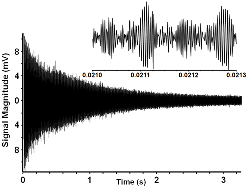
Ion cyclotron resonance time domain signal.
Somewhere in all those lines Ion X is recorded. But you sure can’t tell from what we’re looking at. In order to make any sense out of this picture, we need to descramble the signals, convert them to frequency data and sort them out.
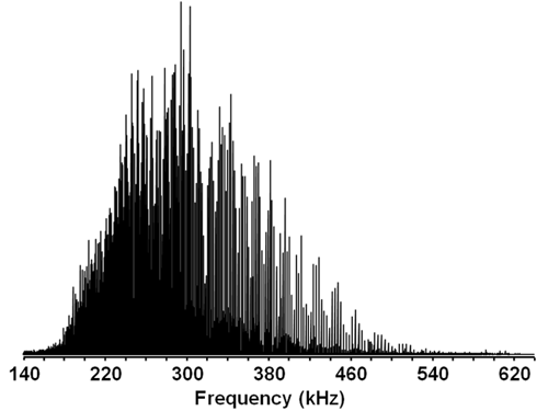
That magic is worked by a mathematical algorithm called a Fourier transform (finally we reach the FT part of our discussion!). A computer converts the raw data from an “amplitude over time” signal to a signal that separates out and depicts the spectrum of all the signals received. Our post-FT data looks like this:
Frequency domain spectrum of crude oil sample.
We’ll spare you the math behind it. For the purposes of understanding FT-ICR, you just need to know that Fourier transform shows you the amplitude of each of the different frequencies detected, which corresponds to the number of ions associated with that frequency.
At last, we come to the final step. The results of the Fourier transform are translated to produce a mass spectrum of our crude oil sample.
Enlarged region of the mass spectrum of a crude oil sample, identifying individual hydrocarbons.
This ought to look familiar – the detailed look of the crude oil sample we studied earlier. And there is Ion X, in the middle of the spectrum, in the neighborhood of 426.30 mass/charge ratio: C28H44N1S1. As it turns out, it's one of several hydrocarbons in the sample containing sulfur (S), and it's a good thing we found it. Sulfur is a strictly regulated pollutant in transportation fuels, and the regulations are getting more strict. So it's increasingly important to identify the molecules that have sulfur and measure how difficult it would be to remove it (a process called desulfurization). A crude oil sample with lots of sulfur molecules that resist desulfurization might not be worth drilling for.
This article has demonstrated just one way in which FT-ICR is used by scientists. Explore the links on the next page to learn more about this powerful and promising process.
Thanks to the Magnet Academy's scientific adviser on this article Chris Hendrickson, Director of Instrumentation in the MagLab's ICR Facility.
By Kristen Coyne